🧠 AI with Python - 📊 Evaluate a Classifier using Confusion Matrix & Accuracy Score

When building a machine learning model, it’s tempting to judge it solely based on accuracy — but accuracy doesn’t always tell the whole story.

That’s where the confusion matrix comes in.

What is a Confusion Matrix?

A confusion matrix is a table that compares the actual vs. predicted classifications made by a model.

• Rows → Actual class labels
• Columns → Predicted class labels

It breaks down predictions into four main categories:

• True Positive (TP) → Correctly predicted positive cases
• True Negative (TN) → Correctly predicted negative cases
• False Positive (FP) → Incorrectly predicted positive cases (Type I Error)
• False Negative (FN) → Incorrectly predicted negative cases (Type II Error)

Why Accuracy Alone Can Be Misleading

Accuracy = (Correct Predictions) / (Total Predictions)

While it’s an easy metric to calculate, it can be deceptive — especially in imbalanced datasets.

For example, if only 5% of your emails are spam, a model that always predicts “Not Spam” will still have 95% accuracy but is useless for detecting spam.

That’s why pairing accuracy with a confusion matrix (and other metrics like precision, recall, and F1-score) is a better approach.

Workflow Overview

Step 1 – Train the Model

We’ll train a Decision Tree Classifier using scikit-learn’s built-in Iris dataset.

from sklearn.datasets import load_iris
from sklearn.model_selection import train_test_split
from sklearn.tree import DecisionTreeClassifier

iris = load_iris()
X_train, X_test, y_train, y_test = train_test_split(
    iris.data, iris.target, random_state=42
)

model = DecisionTreeClassifier(random_state=42)
model.fit(X_train, y_train)

Step 2 – Generate Predictions

After training, we generate predictions for the test set.

y_pred = model.predict(X_test)

Tip: Always use test data (not training data) for evaluation to avoid biased results.

Step 3 – Evaluate with Confusion Matrix & Accuracy Score

We use scikit-learn’s confusion_matrix and accuracy_score to measure performance.

from sklearn.metrics import confusion_matrix, accuracy_score

cm = confusion_matrix(y_test, y_pred)
accuracy = accuracy_score(y_test, y_pred)
print("Confusion Matrix:\n", cm)
print("Accuracy Score:", accuracy)

Output:

Accuracy: 0.9474
Confusion Matrix:
 [[12  0  0]
 [ 0 12  1]
 [ 0  1 12]]

Step 4 (Optional) - Visualize the Confusion Matrix

A heatmap can make the results easier to interpret.

import matplotlib.pyplot as plt
import seaborn as sns

plt.figure(figsize=(5, 4))
sns.heatmap(cm, annot=True, fmt='d', cmap='Blues',
            xticklabels=iris.target_names,
            yticklabels=iris.target_names)
plt.xlabel("Predicted")
plt.ylabel("Actual")
plt.title("Confusion Matrix")
plt.show()

Example Output: Confusion Matrix - Logistic Regression on Iris

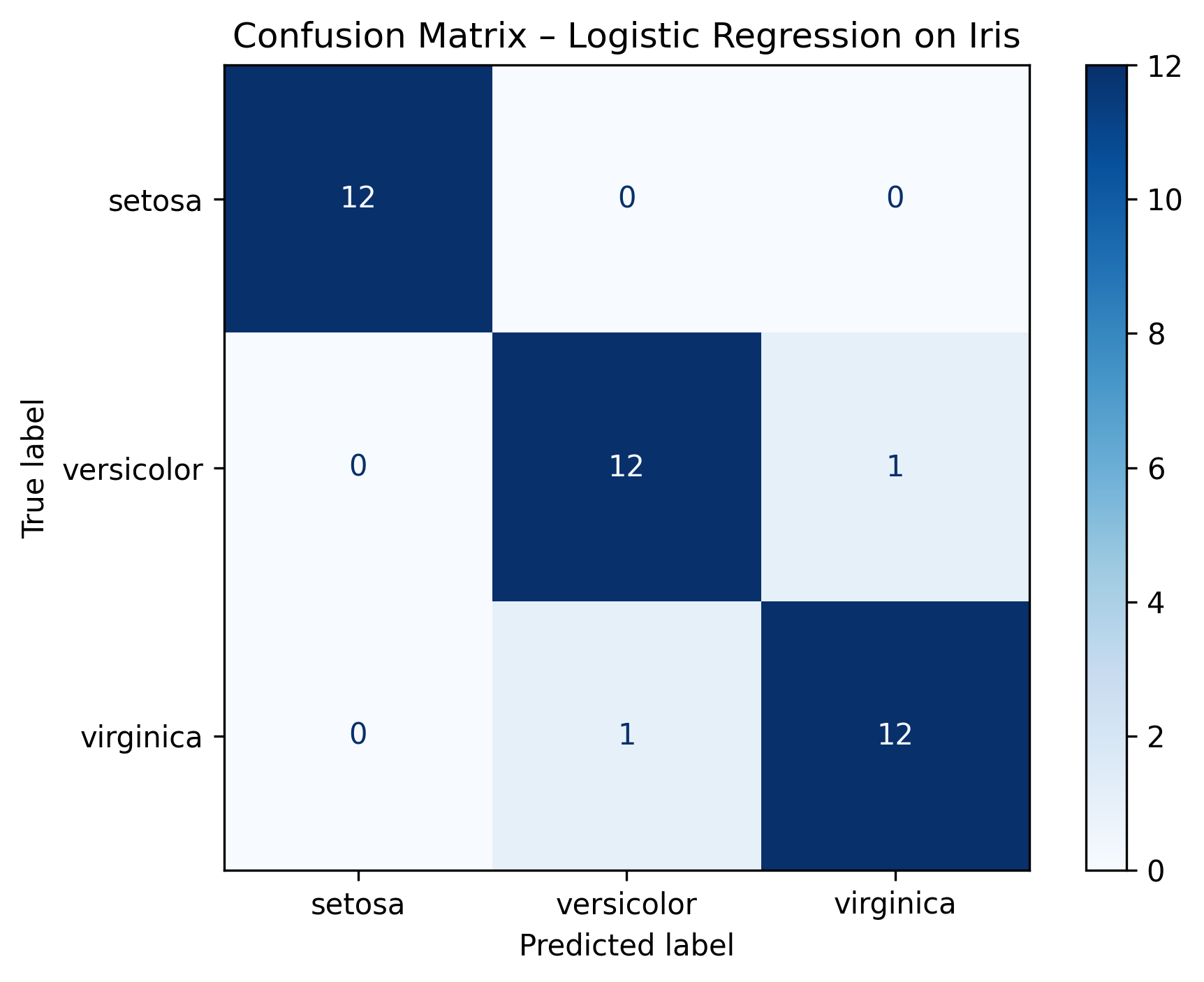
Figure: Confusion Matrix - Logistic Regression on Iris

Practical Use Cases

Confusion matrices are widely used in:

• 📧 Spam Detection → Classify emails as spam/not spam
• 🩺 Medical Diagnosis → Detect diseases with minimal false negatives
• 💳 Fraud Detection → Catch fraudulent transactions without flagging too many legitimate ones
• 💬 Sentiment Analysis → Classify text as positive, negative, or neutral

Pro Tips for Model Evaluation

• Always visualize the confusion matrix (heatmaps make it easier to interpret)
• For imbalanced datasets, focus on precision, recall, and F1-score
• Use classification reports for a complete performance breakdown

Key Takeaways

• Confusion Matrix gives a detailed view of classification performance.
• Accuracy Score is simple but can be misleading if classes are imbalanced.
• Visualization can make interpreting results much easier.